Introduction to Linear Regression

This section will provide a high-level intuitive overview of linear regression and the problem it solves. It serves as a brief context for our gradient calculation sections. As such, a familiarity with the topic of linear regression is welcomed. For more advanced readers this section and a part of the optimization section can be skipped.

Problem statement

To set the stage, a common example of predicting house prices is examined. This represents the first requirement for linear regression use - a dataset. An example dataset is shown below:

The dataset holds the inputs (sqft, bedroom count) and accompanying outputs (price) with respect to the price prediction problem. Let us consider all the input values of an example inside the dataset as a vector $\textbf{x}^{(i)}$. The accompanying output value will be denoted as $y$. We define the dataset with $m$ examples:

$\{( \textbf{x}^{(i)}, y^{(i)})\}_{i=1}^{m}$

Every method of solving a problem carries some assumptions with its use. Linear regression is a method that assumes that the mapping from inputs to outputs is a linear mapping.

Definition: Linear Mapping

Let $V,W$ be real vector spaces , and $f: V \rightarrow W$, then $f$ is a linear map if: $f(\textbf{a} + \textbf{b}) = f(\textbf{a}) + f(\textbf{b})$ $f(\alpha \textbf{a}) = \alpha f(\textbf{a})$

equivalently:

$f(\alpha \textbf{a} + \beta \textbf{b}) = \alpha f(\textbf{a}) + \beta f(\textbf{b})$

With this in mind, we want to define a rough form of functional dependence between inputs and outputs. As seen, we are allowed to multiply and add inputs inside the function. Multiplying inputs with a scalar is also allowed and we will denote these scalars as $\theta_i$. The function w.r.t our two inputs is defined as:

$y = \theta_0 + \theta_1 x_1 + \theta_2 x_2$

This function is the fundamental view of the problem that we operate on under the linear regression lens. Next, the goal of linear regression is to estimate the unknown parameters $\theta_i$ that are particular to our dataset (while retaining a good generalization ability).

Note

Why is $\theta_0$ alone with no $x$? You can view it as if $x_0 = 1$, this way $\theta_0$ represents the bias in our function. Geometrically it removes the constraint that the function must pass through the origin.

More generally, if we had $n$ inputs, we can expand easily:

$y = \theta_0 + \theta_1 x_1 + \theta_2 x_2 + ... + \theta_n x_n$

In a summation form, while respecting $x_0=1$ we can write:

$y = \sum_{j=0}^{n} \theta_j x_j$

Cost

How wrong are we?

Assuming we don’t know how to go about estimating the parameters in our function, we take a wild guess by choosing a vector of parameters $\boldsymbol{\theta}$. How good was this guess? This is a powerful question.

If the dataset contains an entry for a house with $1000$ sqft, $2$ bedrooms, and a price of $200,000$ USD, and our guess parameters produce an output of $150,000$ USD for those same inputs, then we are off by $50,000$ USD. What we just did is measure the error $e$. If we can measure, we can optimize.

Error was computed as the difference between the actual output $y$ and the predicted output $\hat{y}$ $\hat{y} = \theta_0 + \theta_1 x_1 + \theta_2 x_2$ $e = \hat{y} - y$

What if the guess was $250000$ USD? Then the error would be $-50000$ USD. We don’t want the error to be negative so the equation is adjusted with the absolute sign

$e = |\hat{y} - y|$

Successful measurement of the model’s error per example is now possible. Our interest is not in the error the model makes for a single example because we desire a broader generalization ability. To express the error across the entire dataset an average of the errors over all examples is computed in the form of a cost function:

$J = \frac{1}{m} \sum_{i=1}^{m} | \hat{y}^{(i)} - y^{(i)}|$

Should we treat each error the same?

What we have derived is close to the actual cost function that is used in linear regression. Linear regression cost function additionally squares the residuals and divides by $2$. The square operation can be interpreted as a way to penalize large errors more than small ones. The division by $2$, on the other hand, is a mathematical trick that makes the derivative of the cost function easier to compute which we will see later.

Expressing the cost function w.r.t. inputs, outputs, and parameters we obtain:

Origin of the cost function

Even though we intuitively arrived at the cost function, the choice for it is not arbitrary. It can be rigorously derived from statistical principles using maximum likelihood estimation. Maximum likelihood estimation is outside of the scope of this blog post. For more information open page 263. in [1].

Optimization

The best parameters $\theta$ for our model are the ones that minimize our cost function. This requires solving a minimization problem of our cost function with respect to our parameters. There are two approaches to solving this minimization: the iterative and the analytical approach. Both approaches use the concept of a derivative. The derivative of a function tells us the slope of a function at a point. When a derivative of a multivariable function is computed with respect to one of its variables we call it the partial derivative. The significance of it gets more clear if we imagine our cost function as a landscape. If we had only two parameters, we can interpret them as longitude and latitude of the landscape while the elevation would be represented with our cost function. An oversimplified version of this landscape is shown below.

#| echo: false

import plotly.graph_objects as go
import numpy as np

# Define the paraboloid function
def paraboloid(x, y):
    return x**2 + y**2

# Create a grid of x and y values
x_vals = np.linspace(-10, 10, 100)
y_vals = np.linspace(-10, 10, 100)
x, y = np.meshgrid(x_vals, y_vals)

# Calculate z values using the paraboloid function
z = paraboloid(x, y)

# Create a 3D surface plot with surfacecolor mapped to z values
fig = go.Figure(data=[go.Surface(x=x, y=y, z=z, surfacecolor=z, 
                                  colorscale='Jet')])

# Set the axis labels
fig.update_layout(scene=dict(xaxis_title="theta2", yaxis_title="theta1", zaxis_title="J"))

# Show the plot
fig.show()

Knowing the slope at each point with the help of the derivative means knowing in which direction to move should we want to go downhill (minimize the cost). Slope also reveals when a local minimum has been reached as it will equal zero. Iterative approach uses this to make small steps in the downhill direction while the analytical approach solves directly for the derivative being zero.

Iterative solution

As briefly mentioned above, the iterative approach tries to find the minimum by moving downhill in this landscape. When we calculate the derivative for our choice of theta, if the slope is negative we should continue in that direction and if the slope is positive we should move in the opposite direction. We can repeat this process until we reach a minimum.

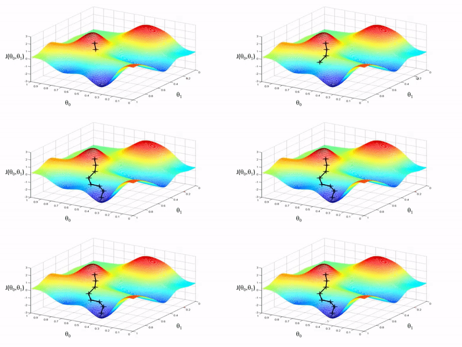
This iterative type of solution is called gradient descent. To perform gradient descent we can start with an arbitrary choice of parameters $\theta$ and define our cost function $J$. For each $\theta_k$ we calculate the partial derivative of the cost function $\frac{\partial}{\partial \theta_k} J$ to get the slope. If the slope is positive that means the minimum is in the opposite direction so we can subtract the slope from $\theta_k$ and if the slope is negative we add the slope to $\theta_k$. This is what the minus symbol is for. Additionally, we multiply the slope by a learning rate $\alpha$ to control how big of a step we take.

$\theta_k := \theta_k - \alpha \frac{\partial}{\partial \theta_k} J$

There are considerations that were left out of this section, specifically the concept of global/local minima, convergence, overfitting, etc. As the goal of this post is to showcase how the gradient is derived, we will leave these considerations aside.

Calculating the derivatives/gradient

Having provided enough context on linear regression we proceed with one of the main goals of this post - the linear regression gradient calculation. A step-by-step approach to gradient calculation follows, along with every important calculus or linear algebra rule that we may require.

Non-vectorized derivative calculation

A non-vectorized calculation of derivatives is performed in this section. First, a list of derivation rules we may need to use are listed below:

We proceed with the step-by-step derivation of the cost function. Since the cost function is multivariable, our derivatives turn into partial derivatives that need to be calculated for each parameter $\theta_{k}$.

Vectorizing the derivation result

Vectorization of our derivation result is performed here. The inner sum can be rewritten as a dot product or a trivial matrix multiplication.

Calculating all the partial derivaties at once can be expressed as calculating the vector of partial derivatives, i.e. the gradient.

Last sum to vectorize is the summation over the dataset. To vectorize we first introduce a matrix $\textbf{X}$ where each row is $(\textbf{x}^{(i)})^T$. Likewise, we introduce $\textbf{y}$ as a vector of outputs. Predictions are now of the form $\textbf{X}\boldsymbol{\theta}$ and the vector of residuals is $\textbf{X}\boldsymbol{\theta} - \textbf{y}$. We are left to take care of our $\textbf{x}^{(i)}$ in the previous equation. Remember that the gradient must be a vector.

Let us first understand what is done in the previous equation with $\textbf{x}^{(i)}$. Our parentheses, when solved, produced a single number, and $\textbf{x}^{(i)}$ was a vector. The summation, therefore, performs a summation over individual scalar vector products. Returning back to our new equation we have a vector of residuals. Each value of that vector needs to multiply the corresponding vector $\textbf{x}^{(i)}$ and all of the results need to be summed. If we transpose $\textbf{X}$ and put it on the left side of the equation we get exactly that.

$\textbf{X}^T(\textbf{X}\boldsymbol{\theta} - \textbf{y})$

Tip

This way, for example, the first row of $\textbf{X}^T$ will be all $x_0$ features of all examples. If that is multiplied by the residual vector $(\textbf{X}\boldsymbol{\theta} - \textbf{y})$ we get a single value, the first value of gradient vector $\nabla_{\boldsymbol{\theta}}J_0$

Our final equation takes the form:

$\nabla_{\boldsymbol{\theta}} J = \frac{1}{m} \textbf{X}^T(\textbf{X}\boldsymbol{\theta} - \textbf{y})$

Vectorized derivative calculation

Vectorization is usually done before any derivation rules are used. In this section we vectorize immediately and apply new derivation rules for the vectorized form.

We will focus on the term without normalization and account for it at the end. Square operation will be split as follows.

Before calculating the gradient, we will list the calculus / linear algebra rules that will be useful.

Gradient calculation follows.

The term $\boldsymbol{\theta}^T\textbf{X}^T\textbf{y}$ is actually a scalar if you consider individual element dimensions. A transpose of a scalar is that same scalar, so a transpose applied to it wouldn’t change anything but it would simplify our equation.

We take a look at each gradient individually:

We obtain:

Accounting for the normalization we arrive at our previous conclusion:

Analytical Solution

Analytical solution to linear regression does not perform gradient descent. Instead, it searches for a solution to the normal equation, i.e. it sets the cost function gradient to zero and solves for $\boldsymbol{\theta}$

$\textbf{X}^T(\textbf{X}\boldsymbol{\theta} - \textbf{y}) = 0$

How can we be sure that this exact solution exists? This refers to the concept of local or global minima. Some functions can have multiple minima and finding the global one is hard. Iterative approaches shine in this case (under considerable adjustments) and are the backbone of every major neural network model training. What can be said about our function? It would be ideal if our function had a single global minimum. Function of that type is called a convex function.

Definition: Convexity

A function $f:(a,b)\rightarrow \mathbb{R}$ is convex if for all $x_1,x_2\in(a,b)$ and $\lambda_1,\lambda_2 \ge 0$ such that $\lambda_1 + \lambda_2 = 1$, $\lambda_1 f(x_1) + \lambda_2 f(x_2) \ge f(\lambda_1 x_1 + \lambda_2 x_2)$

If $f$ is differentiable and $f^{\prime\prime}(x) \ge 0$ for all $x\in(a,b)$, then it is convex. It is strictly convex if $f^{\prime\prime}{x}>0$

For vector inputs if the function is twice differentiable, that means the Hessian exists for all values in the domain of x. then the function f(x) is convex if and only if $\nabla_{x}^2 f(x)$ is positive semidefinite

A symmetric matrix A is positive definite if for all non-zero vectors $b \in \mathbb{R}^n$, $b^TAb > 0$.

A symmetric matrix A is positive semidefinite if for all vectors $b \in \mathbb{R}^n$, $b^TAb \ge 0$.

Turns out our function is indeed convex, let us prove that.

If we plug $A = \textbf{X}^T\textbf{X}$ it into our positive semidefinite definition we get

$b^TAb = \textbf{b}^T\textbf{X}^T\textbf{X}\textbf{b}$

The term we obtain is a squared euclidean ($l_2$) norm. It is zero only when $\textbf{b}=0$ or $\textbf{X}\textbf{b} = 0$, else it is positive. We can conclude that our cost function is convex. With this out of the way, we set gradient to zero and solve for $\boldsymbol{\theta}$

$\nabla_{\boldsymbol{\theta}} J = \frac{1}{m} \textbf{X}^T(\textbf{X}\boldsymbol{\theta} - \textbf{y})$

We arrived to the closed-form equation that gives us the solution.

Disclaimer about the inverse

This solution is showcased in most of the textbooks and online courses but is not used in practice. Reason is that the inverse of $\textbf{X}^T\textbf{X}$ doesn’t always exist. This inverse doesn’t exist when there are redundant features (two features are linearly dependent) or when there are too many features ($m \le n$).

Frameworks like numpy inside their linear regression implementations (e.g. np.linalg.lstsq) use a different kind of an inverse to solve these edge cases - the pseudoinverse. Pseudoinverse is always defined and is obtained by a standard matrix factorization technique called singular value decomposition (SVD). Pseudoinverse is outside the scope of this post.

References

Useful resources for exploring the topic of linear regression in more detail are listed below.

• [1] Book, Mathematics for Machine Learning by Marc Peter Deisenroth, A Aldo Faisal, and Cheng Soon Ong
• [2] Notes, CS229 lecture notes by Stanford
• [3] Course, Machine Learning course by Stanford on Coursera
• [4] Course, Mathematics for Machine Learning by Imperial College London on Coursera
• [5] Notes, Computing Neural Network Gradients by Kevin Vlark