
My winning solution to FERIT Osijek’s 2022 Rock-Paper-Scissors-Lizard-Spock (RPSLS) competition, which took 1st place with a score of 1942/2000. The approach was a small LSTM that learns the opponent’s behavior while the match is still being played, predicts its next move, and plays the counter.
The competition
Entrants wrote a player algorithm that plays 2000 consecutive games of RPSLS against an unknown robot algorithm. Each game both sides pick a move at the same time, and the winner takes a point; draws score nothing for either side. The highest total after 2000 games wins. Critically, the rules let both sides use the complete history of the opponent’s past moves, plus “random selection functions and any mathematical functions”, to decide what to play next. That last clause is the whole problem, and I will come back to it.
The competition also used its own ruleset rather than the familiar Big Bang Theory one. Here scissors beats paper, paper beats rock, rock beats scissors, all three beat lizard, and Spock beats everything except lizard, which beats Spock. That asymmetry matters more than it first appears. Counting how many moves each one beats, Spock wins against three of the five and loses only to lizard, so against an opponent picking uniformly at random Spock alone wins about 60% of games. Lizard is the mirror image: it beats only Spock and loses to the other three, making it the weakest move on its own and the only answer to Spock.
That gives two useful baselines to measure against. A player choosing uniformly at random scores roughly 800 out of 2000. A player who simply hammers Spock every single game scores roughly 1200 against a random opponent. The winning submission scored 1942.
Why the obvious approaches cap out
The natural first attempt is frequency counting: track what the opponent has played most often and counter it. That handles a robot with a fixed bias and nothing else. The next step up is conditioning on the opponent’s last move, which beats the large family of robots that react to what you just did.
Neither touches the robots that key off the game index rather than the move history. A robot whose logic is essentially “play rock when the game number is divisible by 10, Spock otherwise” produces a move sequence that looks close to noise if the only thing fed to the model is past moves. There is no pattern in the move stream to find, because the pattern lives in the clock, not in the play. The rules explicitly permitted “any mathematical functions”, so I had to assume the opponent used them.
Predicting the opponent instead of picking a move
I framed the task as sequence prediction rather than learning a policy directly. The model never learns what I should play. It learns to predict what the robot will play next, and a small deterministic lookup then picks a move that beats that prediction. Keeping those two responsibilities apart made the model much easier to reason about: if my score was poor I could ask whether the prediction was wrong or the counter logic was wrong, and check them separately.
The counter table is the one piece encoding the competition’s specific rules. When more than one move beats the prediction it picks between them at random, which costs nothing and makes my own play harder to model in return.
Teaching the model to see the clock
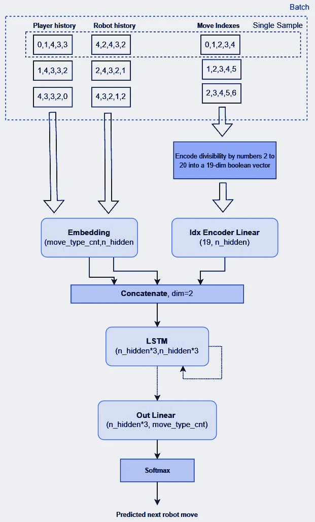
The idea that actually won the competition was giving the model the game index as a feature, encoded so it could express periodicity. At each position I take the game number and turn it into a 19-dimensional boolean vector recording whether it divides evenly by each of 2 through 20.
This is what lets an index-based opponent become learnable. A robot keyed on i % 10 shows up as a clean, perfectly correlated signal in the “divisible by 10” slot. One keyed on i % 3 or i % 7 shows up in its own slot. The model does not need to discover modular arithmetic from scratch, which a small LSTM on a few hundred samples has no realistic chance of doing. It only needs to notice that one of nineteen boolean channels lines up with the opponent’s behavior. Handing the network the right representation did far more work here than any amount of capacity or training time would have.
The model
The architecture is deliberately small, because the entire training set is whatever moves have been played so far in the current match.
Both players’ move histories go through a shared 5-token embedding of width 32, so my moves and the robot’s are represented in the same space. The 19-dimensional divisibility vector goes through its own linear encoder to the same width. The three are concatenated into a 96-dimensional sequence, run through a single-layer LSTM with a 96-unit hidden state, and projected back down to five logits with a softmax over the possible moves.
Training against an opponent while playing it
Because the data only exists once the match is under way, training happens during the game. The first 50 moves are played without a model at all, purely to accumulate history.
From there I cut the history into overlapping windows of 16 moves with a stride of 1, and deliberately do not shuffle them. The train and validation split is chronological, 80/20, so validation always measures prediction on games that happened after the ones trained on. Shuffling would have leaked future behavior into the training set and produced a validation loss that looked good and meant nothing.
Two details mattered for squeezing signal out of so little data. The loss is computed at every position in the window rather than only the final one, so a single 16-move window contributes 16 supervised predictions instead of one. And training restarts from scratch at a fixed schedule of games (50, 100, 150, 200, 300, 500, 800 and 1000) rather than being fitted once. A model fitted early tends to become confidently wrong when the opponent’s behavior shifts, and rebuilding it periodically is a blunt but effective way to stay current. Each run uses Adam at a learning rate of 1e-3, batches of 64, and early stopping with a patience of 3 on validation loss, with a hard stop once loss falls below 1e-4 so training never eats the time budget.
Knowing when not to trust the model
The model does not get to play every move. Its softmax confidence has to clear 0.8 before I act on the prediction; below that I fall back to a random move. Against a genuinely random opponent the model never becomes confident, so this gate stops it from converting an unpredictable opponent into a stream of confidently wrong guesses.
The fallback itself is not uniform: it is weighted 50% Spock, 20% lizard, and 10% each to scissors, rock and paper. That skew matters because of the ruleset. Spock is the strongest single move and lizard is the only thing that answers it, so even when the model has nothing useful to say, the fallback is still playing a better-than-even game rather than flipping a five-sided coin.
Testing against sixteen opponents
I could not see the competition robot, so I wrote sixteen of my own and built a benchmark harness that runs a full 2000-game match against each and reports wins, draws and losses. They span the strategy families I thought plausible: reactive robots that counter my previous move, a mirror that simply copies it, a uniform random baseline, robots that reach further back into history at fixed depths, and a group built entirely on the game index using i % 10, i % 3, i % 5 and i % 7.
That last group is the reason the divisibility encoding exists. Hyperparameters were tuned by searching against this benchmark set, then hardcoded for submission, since the submission had to run standalone with no opportunity to tune against the real opponent.
What I would do differently
Retraining from scratch on a fixed schedule is wasteful and arbitrary. A better version would detect distribution shift, by watching prediction accuracy over a rolling window, and retrain when the opponent’s behavior actually changes rather than when a counter hits a preset number. The confidence threshold is similarly a single hardcoded value that would be better calibrated against observed accuracy as the match progresses. The benchmark harness was already in place to evaluate either change.
Related reading
View the full code on GitHub →