
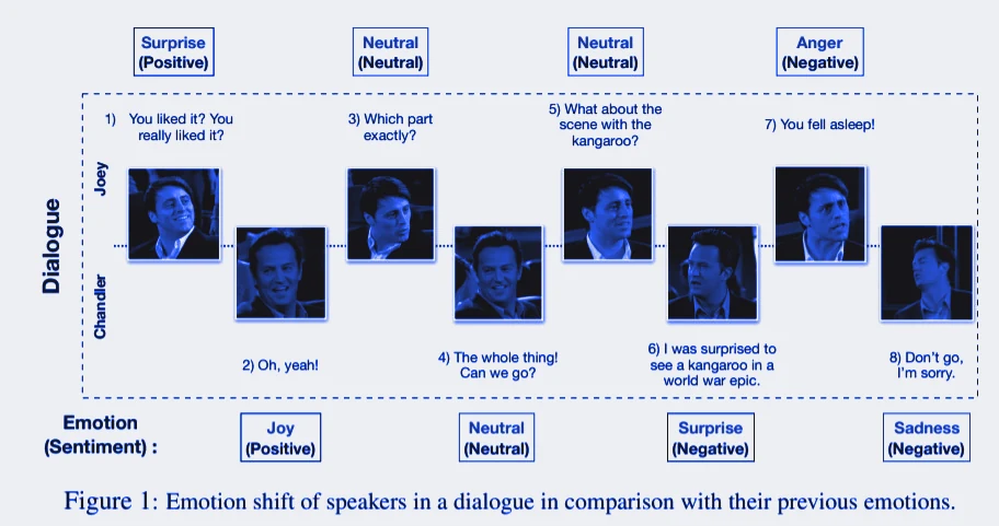
Figure 1 from MELD: A Multimodal Multi-Party Dataset for Emotion Recognition in Conversations, Poria et al. (2018), which introduced the dataset used here.
A model that predicts a speaker’s emotion from what they said and how they said it, built at the PSI:ML7 Machine Learning Institute by Brando Koch and Nikola Andrić Mitrović under the supervision of Tamara Stanković from Microsoft, and trained on the MELD dataset.
The task
MELD is built from dialogues in Friends. Every utterance comes with the text, the audio, and a label from seven emotions, and it sits inside a conversation rather than on its own.
That context is what makes the problem harder than ordinary sentence classification. A speaker’s emotion shifts turn by turn depending on what was just said to them, so the same sentence can be neutral in one exchange and angry in another. Text alone also loses a lot. “Oh, great” is sarcasm or enthusiasm depending entirely on delivery, and only the audio settles it.
Getting the data into shape
MELD ships as video clips with a CSV of utterances beside them, so the audio has to be extracted before any of it is usable. A preprocessing step pulls a wav out of every clip and writes it into per-split folders, which keeps the expensive decode out of the training loop entirely.
At load time each wav is read, downmixed to mono by averaging across channels, and resampled to 16 kHz. Padding happens per batch rather than to one global maximum: the collate function pads every waveform in a batch up to the longest one in that batch. Utterances in MELD range from a word to several seconds, so padding globally would push a large amount of silence through the convolutions on most examples and waste most of the compute.
The text side tokenizes to a vocabulary of ten thousand and truncates at 128 tokens, with GloVe 6B 100-dimensional vectors available to initialise the embedding rather than starting it from noise. Exploratory notebooks for each modality sit alongside the training code, which is where the class balance and the utterance-length distribution were checked before any model was written.
Two encoders, joined late
Text and audio run through separate encoders and only meet near the end.
The text encoder embeds tokens into 100 dimensions, runs them through an LSTM of the same width, applies dropout at 0.2, and then takes both the average and the maximum of the outputs across time and concatenates the two. Taking only the final hidden state throws away most of the sequence, and pooling both ways keeps a summary of the whole utterance alongside its strongest signal. Concatenating the two pools is what makes the text vector 200 wide rather than 100.
The audio encoder is an M5 convolutional network that works on the raw waveform. The first convolution is wide and strided, 80 samples with a stride of 16, and produces 32 channels. Three narrower convolutions follow with a kernel of 3, widening to 32, 64 and 64 channels, each with batch normalization, a ReLU and a max pool of 4. A global average pool over the time axis collapses whatever is left into a single 64-dimensional vector, so clips of different lengths all come out the same size.
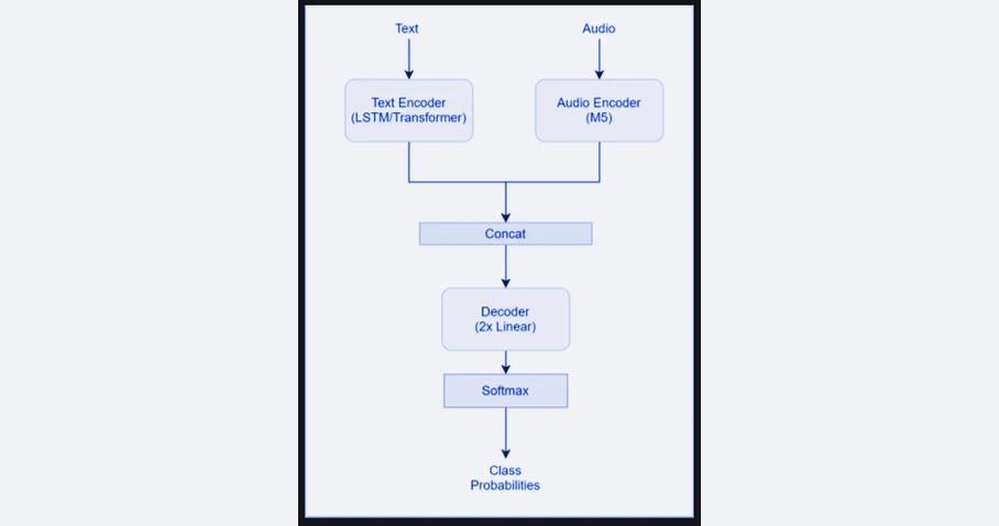
Those two vectors are concatenated into 264 and passed through a linear layer down to 100, a ReLU, and a final linear layer to the seven emotion classes. Joining late like this means each encoder learns its own modality without interference, and the decoder only has to learn how much to trust each one.
MELD ships two label sets, three-way sentiment and seven-way emotion, and several of the single-modality baselines predict the coarser three while the multimodal model predicts all seven. The coarse task is a useful sanity check on an encoder before asking it to separate anger from disgust.
Skipping the spectrogram
Most audio classification starts by turning the waveform into a mel spectrogram and treating it as an image. That is not the approach here.
The first convolution has a kernel of 80 samples with a stride of 16, applied directly to audio resampled to 16 kHz. At that rate a kernel of 80 covers five milliseconds, so the layer is learning its own filterbank from the raw signal instead of using a fixed one chosen in advance. The rest of the stack widens the receptive field with pooling until a single vector covers the whole clip.
The tradeoff is that raw audio needs more data and more compute than spectrograms to reach the same place. It is worth it here mostly as an experiment, and because it removes one preprocessing decision that would otherwise be baked in before the model sees anything.
The choice came out of trying three audio front ends. The first flattens the input and pushes it through four fully connected layers with batch normalization and heavy dropout, which is the obvious baseline and also the one that ignores time entirely. The second is a two-dimensional convolutional stack of the kind you would point at a spectrogram, six conv layers halving the resolution each time. The third is M5 on the raw signal, and it is the one that ended up in the multimodal model.
Two versions of the text encoder
The text side is built twice, so the two can be compared under identical conditions.
The first uses the LSTM described above. The second replaces it with a transformer encoder: two layers, a single attention head, a feed-forward width of 100, dropout at 0.25, and sinusoidal positional encoding added to embeddings scaled by the square root of the model dimension. Both feed the identical audio encoder and the identical decoder, so a sweep can pick between them as just another hyperparameter rather than the choice being guessed up front.
A BERT baseline on text alone runs in a separate notebook, to show how far a pretrained model gets without any of this. That is the honest comparison for a from-scratch encoder, and it is worth having even when the answer is unflattering.
Searching the hyperparameters
Training is wired to Weights and Biases with Bayesian sweeps rather than a grid.
The sweep moves over learning rate and weight decay on log-uniform ranges, the one-cycle maximum learning rate, batch size, epoch count, text sequence length, and which of the two models to use. Optimising for validation loss and letting the search decide between architectures is a lot more honest than picking one first and tuning it, since the better architecture under one set of hyperparameters is often not the better one under another.
The defaults the sweep starts from are batch size 128, fifty epochs, Adam with weight decay, and a one-cycle schedule, with the text truncated to 128 tokens and a vocabulary of ten thousand. Audio is downmixed to mono, resampled to 16 kHz, and padded per batch rather than to a fixed global length, so short utterances do not carry a tail of zeros through the convolutions.
The training loop sits on a learner-and-callback structure, which keeps the loop, the logging and the metric tracking separate from the models themselves and lets a sweep swap architectures without touching either.
View the code on GitHub → · MELD dataset · MELD paper