
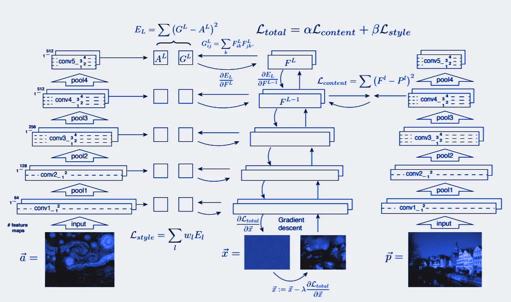
A from-scratch PyTorch implementation of “Image Style Transfer Using Convolutional Neural Networks” by Gatys, Ecker, and Bethge (CVPR 2016). I wrote it to sit as close to the paper as an implementation reasonably can: layer names follow the paper’s notation rather than the framework’s, docstrings quote the passages they implement, and the shipped defaults reproduce the paper’s own figures instead of an unrelated demo.
Optimizing the image instead of the network
The thing being trained here is the picture, not the model. A pretrained VGG19 is loaded, switched to eval mode, and has every parameter frozen, so nothing about the network changes during a run. The tensor I hand to the optimizer is a block of white noise shaped like the content image, and it is the only thing in there, so backpropagation runs the whole way through the frozen network and lands on the pixels themselves. Each step nudges those pixels toward a lower loss, and over a run the noise resolves into the output image.
Optimization uses L-BFGS, as the paper does, driven through a closure that clamps the image back into the valid [0, 1] range before every evaluation, since unconstrained pixels drift out of range and visibly degrade the result. The default iteration count of five looks far too low until L-BFGS is accounted for, since it makes many internal function evaluations per step, building a curvature estimate rather than taking a single gradient step the way SGD would.
Representing style as feature correlations
Content is the straightforward half: take the activations of one layer, reshape them to a matrix of filters by spatial positions, and two images match in content when those activations match.
Style has to survive being moved around the frame, which rules out anything positional. The paper’s answer, and what this implements, is the Gram matrix: multiply a layer’s activation matrix by its own transpose, so that entry (i, j) becomes the inner product of feature map i with feature map j across the whole image. It records which filters tend to fire together and discards where they fired, which is precisely the split needed to lift a painter’s brushwork and palette off their canvas without dragging the scene along with it. Style is read from five layers at once, conv1_1 through conv5_1, because texture lives at several scales simultaneously, while content is read from a single deeper layer.
Normalizing the style loss across layers
Gram matrices from different layers arrive at wildly different magnitudes, because a deep layer with 512 filters over a small spatial map produces far larger inner products than an early layer with 64 filters over a large one, and left alone a single layer dominates the entire style term. I walk the style image through the network once before optimization begins and record the filter count and the spatial extent of every style layer, then scale each layer’s contribution by one over four times the squared filter count times the squared spatial extent, which is the normalization the paper specifies. The five scaled losses are averaged with equal weight. Because the style image never changes during a run, all of this is computed once up front rather than every iteration.
Total loss is a linear combination of the two terms, content weighted by alpha and style by beta, shipped at 1 and 1e7 respectively. That ratio looks extreme until the normalization constants above are taken into account.
Following the paper down to the details
Four choices carry most of the fidelity. Torchvision exposes VGG19 as a flat indexed list of layers while the paper talks in terms of conv4_2 and relu3_1, so I carry an explicit map between the two, all thirty-seven entries, which means a layer can be selected by the name the paper gives it. Every max pooling operation in the network is replaced with average pooling on construction, a one-line change whose docstring quotes the paper’s own finding that average pooling yields slightly more appealing results for image synthesis. Inputs are normalized to ImageNet statistics, since that is the distribution the pretrained weights expect. And the bundled images are the paper’s own: the Tübingen Neckarfront photograph as content, with styles by Van Gogh, Munch, Picasso, Kandinsky, and Turner, so running the defaults reproduces the figures rather than something incidental.
Content and style reconstruction from the same code
Because the two loss terms are independent, zeroing either weight turns the same program into a different experiment. Dropping the style weight to zero leaves only the content objective, and the noise resolves into a reconstruction of the content image whose fidelity reveals how much spatial detail the chosen layer actually retains, which is the paper’s demonstration that deeper layers encode content rather than pixels. Dropping the content weight to zero instead gives pure texture synthesis, the style image’s brushwork and palette with no scene in it at all. All three modes ship as one-line shell scripts differing only in those two numbers.
Reproducible outputs
I have every run write two files sharing a timestamp: the generated image, and a log containing the complete argument set as JSON, covering both source images, the dimensions, both weights, the exact layer names, the iteration count, and the optimizer. Every example image in the repository can therefore be regenerated from the file sitting beside it. Given how sharply the result swings with layer choice and with the content-to-style ratio, an output image without its settings is close to worthless, and this is the cheapest possible way to avoid that.
Released under an MIT license.
View the full code on GitHub → · Read the paper (CVPR 2016) · Related: Transformer paper from scratch · PyTorch sequence models